Grokking Modular Addition

Grokking Modular Addition#

Dani Balcells, April 2nd 2024

Introduction#

A few weeks ago, a bunch of us at Recurse Center finished going through most of the materials for the ARENA course, which Changlin Li kindly walked us through. Régis Schiavi and I decided to keep working on one of the optional tracks - replicating the results of the 2023 paper by Neel Nanda et al. titled “Progress Measures for Grokking Via Mechanistic Interpretability”. For several reasons, this bit of work felt like a step up in difficulty compared to the rest of the course, so it felt worth writing a blog post about.

This notebook borrows heavily from the ARENA course contents, specifically from the section on grokking and modular arithmetic.

Setup#

Motivation: what is “grokking”?#

The main reason we conduct this study is to explore the concept of “grokking” in neural networks—the modular arithmetic task, which we’ll explain in detail in the next section, just happens to offer a convenient way to study grokking.

But what is grokking? Let’s take a step back and consider the concepts of generalization and overfitting, which are central to virtually all forms of supervised machine learning. In supervised learning, we have a set of labeled examples (for example, pictures of animals labeled “cat”, “dog”, “parrot”) and we train an model to correctly map inputs to labels. Critically, though, we want it to be able to perform this task not only on the data we use during the training process, but also on new data—we want it to be able to generalize. Unfortunately, if we’re not careful, our algorithm will simply memorize the labels for the training set instead of learning a general rule, leading it to perform well on the training set but not on new data—we call this overfitting. A common way to avoid overfitting is to hold back part of our labeled data in a test set, which isn’t used to update the model’s parameters during training, and instead is only used to measure the model’s performance on unseen data (i.e. its ability to generalize).

In many common and desirable training scenarios, performance on the test set often roughly follows performance on the training set. This often indicates that the model is indeed learning a general rule, and performs only slightly worse on unseen data than on training data.

However, recent experiments have shown an unusual relationship between training and test loss in some scenarios. In an initial phase, loss on the training set drops quickly while loss on the test set remains high, suggesting that the model has “memorized” the relationship between inputs and outputs instead of learning a general rule. When confronted with this behavior, we’d perhaps assume the training isn’t working, and start over after making some changes in the design of our model or training process. It turns out, though, that in some cases, as in the modular addition case, if given just the right amount of training data, after a considerable number of training epochs (about 10,000 in our case) during which training loss remains low and test loss remains high, test loss suddenly drops, indicating that the model has learned a general rule long after memorizing the training set. We call this sudden generalization long past the point of memorization “grokking”.

This behavior is puzzling, and prompts a number of intriguing questions: Why does the model generalize so far past the point of memorization? If the training loss is already near zero, what pushes the model to keep learning until it reaches a general solution? How does the transition from a memorized solution to a general one take place at the level of individual parameters and circuits inside the model?

It also has interesting implications from the safety point of view, as it exemplifies emergent behavior in deep learning models: qualitative leaps in capability that appear suddenly over a relatively short number of training epochs. Emergent behavior and this sort of phase change during training are examples of the “more is different” principle in machine learning, which describes how continuous, quantitative progress can lead to sudden, qualitative differences in outcomes and capabilities. This is important from a safety perspective because it makes it hard for us to predict future capabilities by linear extrapolation of current capabilities. What if, for example, self-perception or the ability to deceive were also emergent properties that arise in phase shifts? A better understanding of grokking might help us shed light on these questions.

The task: grokking modular addition#

The task we’re focusing on in this post is modular addition: $z = (x + y) \% p$, that is, the residue of dividing $x + y$ by $p$. For example, $(70 + 50 )\% 113 = 120 \% 113 = 7$.

In our setup, the model learns a fairly constrained version of this problem: we’re fixing p to the value 113, and we’re limiting x and y to the integers between 0 and 113.

The model we are reverse-engineering is a transformer with a single layer, with four attention heads, no layer norm, d_model = 128, and d_mlp = 512. The diagram below is taken from the ARENA materials.

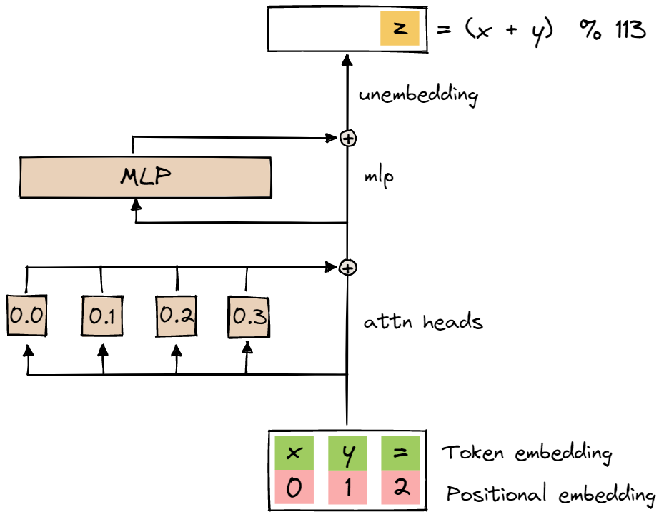
The model takes sequences of three one-hot encoded vectors as inputs: the first two correspond to the one-hot encodings of the inputs x and y, and the third one corresponds to the one-hot encoding of =. Each one-hot encoded vector has length p+1, allowing us to represent the integers between 0 and p-1, plus the token =.

The model outputs three logit vectors, one for each element in the input sequence. The p values in each logit vector represent a probability distribution over the integers between 0 and p-1.

We keep only the output token predicted for input token = as the result of the modular addition operation, that is, we feed the three-element input sequence forward through the transformer, and take only the last (i.e. the third) token of the output sequence as the result of the operation. We train the model on the cross-entropy loss between the logits for this last output token and the one-hot encoding of the correct result of the modular addition.

Note that both one-hot encoded inputs and logit outputs represent distributions over the discrete and relatively limited space of the integers between 0 and p-1. This means that we’re effectively treating the modular addition task as a classification task, from discrete and limited inputs to discrete and limited outputs. The general case of learning modular addition for two continuous and arbitrary inputs is far more complex and beyond the scope of our study, which is primarily concerned with grokking rather than modular addition.

Training is done by generating the full set of [x, y, '='] sequences for all values of x and y between 0 and p-1. Note that, for this toy model, the entire input space is fairly small—there are only $p \cdot p = 12,769$ possible inputs. We train on full batches, using 30% of the total sequences for our training set. We use AdamW with very high weight decay (wd = 1). Weight decay plays an important role in grokking, as we will later see.

Loading the model#

The code below defines a HookedTransformer for our task as described above, and loads in the data from the entire training process.

p = 113

cfg = HookedTransformerConfig(
    n_layers = 1,
    d_vocab = p+1,
    d_model = 128,
    d_mlp = 4 * 128,
    n_heads = 4,
    d_head = 128 // 4,
    n_ctx = 3,
    act_fn = "relu",
    normalization_type = None,
    device = device
)

model = HookedTransformer(cfg)
large_root = Path('large_files')

if not large_root.exists():
    os.mkdir(large_root)

from huggingface_hub import hf_hub_download
REPO_ID = "callummcdougall/grokking_full_run_data"
FILENAME = "full_run_data.pth"

hf_hub_download(
    repo_id = REPO_ID,
    filename = FILENAME,
    local_dir = large_root,
)
full_run_data_path = large_root / FILENAME
full_run_data = t.load(full_run_data_path, map_location=device)
state_dict = full_run_data["state_dicts"][400]

model = load_in_state_dict(model, state_dict)

Visualizing the grokking curve#

We can plot the loss over the train and test datasets to view the characteristic “grokking” curve: train loss drops below 1e-6 in just over 1,000 training epochs, while test loss remains essentially unchanged (or even slightly worse). Shortly before the 10,000 epoch mark, however, test loss begins to drop sharply, also going below 1e-6 at around 14,000 epochs. Why could be causing this?

lines(
    lines_list=[
        full_run_data['train_losses'][::10], 
        full_run_data['test_losses']
    ], 
    labels=['train loss', 'test loss'], 
    title='Grokking Training Curve', 
    x=np.arange(5000)*10,
    xaxis='Epoch',
    yaxis='Loss',
    log_y=True
)

Looking around: everything is periodic!#

Using the input space to look inside the model#

We start by running all possible inputs through the model, and capturing all internal variables in a cache.

all_data = t.tensor([(i, j, p) for i in range(p) for j in range(p)]).to(device)
labels = t.tensor([fn(i, j) for i, j, _ in all_data]).to(device)
original_logits, cache = model.run_with_cache(all_data)
# Final position only, also remove the logits for `=`
original_logits = original_logits[:, -1, :-1]
original_loss = cross_entropy_high_precision(original_logits, labels)
print(f"Original loss: {original_loss.item()}")

Original loss: 2.0160624103482405e-07

Using the transformer_lens library, we can access all activations and intermediate variables in the transformer for any input in our batch.

We start by having a look at the attention scores. Since, as described earlier, we only keep the logits for the final token in the output sequence, we index into the attention scores to consider only the attention paid by the final token to all tokens in the sequence (including itself), for each attention head, and averaged across all input sequences.

As the plot below shows, for all four attention heads, the final token = pays no attention to itself, and pays equal attention to the first two input tokens x and y . This makes intuitive sense: the third and final token = holds no useful information before the attention layer, whose job is precisely to move information from the other input tokens to the final position. Since addition is commutative, it makes sense that both x and y inputs get weighted equally by the attention layer.

attn_p = cache['blocks.0.attn.hook_pattern'][:,:,-1,:]
print(f'{attn_p.shape=}')
mean_final_pos_attn = attn_p.mean(0)
print(f'{mean_final_pos_attn.shape=}')
imshow(mean_final_pos_attn, xaxis='Position in input sequence', yaxis='Attention head no.',
       title='Attention paid by final token to each token (average across all input)')

attn_p.shape=torch.Size([12769, 4, 3])
mean_final_pos_attn.shape=torch.Size([4, 3])

Now, for the conceptual leap that I found the most interesting (and hard to grok myself) in this whole exercise. Remember that we’ve fed the entire input space through the model, a total of 12,769 (or $p^2$ for $p=113$) input sequences [x, y, '='] for all possible values of x and y between 0 and 112 (or $p-1$). What if we took our batch dimension, of size 12,769, and rearranged it into two separate dimensions, each of size 113? This would allow us to consider, for example, the value of a certain neuron activation, instead of as a single vector $a_i$ of 12,769 values, as a 113x113 matrix $a_{xy}$ representing the same values as a function of the inputs x and y.

Why bother doing this? You’ll see that things get very interesting when we rearrange activations and attention scores this way.

For example, as you can see below, the activations of the first three neurons in the MLP all follow very periodic patterns as functions of the inputs x and y.

# Take MLP activations from cache
neuron_acts_post = cache['blocks.0.mlp.hook_post'][:, -1, :]
neuron_acts_pre = cache['blocks.0.mlp.hook_pre'][:, -1, :]

# Rearrange batch dimension (p^2) into two separate dimensions p, p
neuron_acts_post_sq = einops.rearrange(neuron_acts_post, "(x y) d_mlp -> x y d_mlp", x=p)
neuron_acts_pre_sq = einops.rearrange(neuron_acts_pre, "(x y) d_mlp -> x y d_mlp", x=p)

top_k = 3
inputs_heatmap(
    neuron_acts_post_sq[..., :top_k], 
    title=f'Activations for first {top_k} neurons',
    animation_frame=2,
    animation_name='Neuron'
)

The same is true for attention scores, as you can see below. Note that we’re plotting only the attention paid by the final token to the token at position 0. As we saw earlier, the attention scores for positions 0 and 1 are almost identical (they are both close to 0.5, while the attention score for position 2 is 0). We can therefore expect (and verify) that the attention paid by the final token to the token at position 1 is a very similar periodic function of the inputs x and y.

attn_mat = cache['blocks.0.attn.hook_pattern'][:, :, 2, :]

attn_mat_sq = einops.rearrange(attn_mat, "(x y) head seq -> x y head seq", x=p)

inputs_heatmap(
    attn_mat_sq[..., 0], 
    title=f'Attention score for heads at position 0',
    animation_frame=2,
    animation_name='head'
)

We can also follow linear paths within the transformer to see how each input token contributes to the input of a given neuron. Looking at the OV circuit, we take the tensor product $W_E \cdot W_V \cdot W_O \cdot W_{in}$ (i.e. the product of the embedding, attention head value, attention head output, and MLP input matrices), which gives us an effective tensor $W_{neur}$ of shape (d_head, p, d_mlp). We can think of this as a (p, d_mlp) matrix for each attention head, whose i-th column represents the contribution to the i-th neuron’s input as a function of the input token. Note that we’re not counting attention weights here. Again, we see that the model exhibits very periodic behaviors: attention weighting aside, as the value of the model’s inputs increases, the inputs to the MLP cycle through a certain periodic function.

# Get weight matrices from the model
W_O = model.W_O[0] # 0-th element here refers to the W_O matrix of the 0-th layer
W_V = model.W_V[0]
W_E = model.W_E[:-1]
W_in = model.W_in[0]

# Calculate effective matrix W_neur
W_neur = W_E @ W_V @ W_O @ W_in
print(f'{W_neur.shape=}')

top_k = 5
animate_multi_lines(
    W_neur[..., :top_k], 
    y_index = [f'head {hi}' for hi in range(4)],
    labels = {'x':'Input token', 'value':'Contribution to neuron'},
    snapshot='Neuron',
    title=f'Contribution to first {top_k} neurons via OV-circuit of heads (not weighted by attention)'
)

W_neur.shape=torch.Size([4, 113, 512])

Similarly, we can turn to the QK circuit and see that it also exhibits periodic patterns. First, we define the effective matrix $W_{attn}$ as the tensor product $r_{final\_pos}\cdot W_Q \cdot W_K^T \cdot W_E^T$, where $r_{final\_pos} = W_E (=) + W_{pos}(2)$ is the initial value of the residual stream at the final position, i.e. the embedding for the = token plus the positional embedding for position 2. This effective matrix, when multiplied on the right by a given input token a, gives us the attention score paid to token a by the = token in position 2. We’re essentially taking the matrix $v \cdot W_Q \cdot W_K^T \cdot w$, which gives us the attention score between the embedding vectors $v$ as query and $w$ as key, and establishing the query vector as the token = in position 2.

We again see that the attention scores are periodic functions of the input token.

# Get weight matrices from model
W_K = model.W_K[0]
W_Q = model.W_Q[0]
W_pos = model.W_pos
# Get query-side vector by summing the embedding for the '=' token plus the positional embedding for position 2
final_pos_resid_initial = model.W_E[-1] + W_pos[2]

# Calculate effective matrix W_attn
W_QK = W_Q @ W_K.mT
W_attn = final_pos_resid_initial @ W_QK @ W_E.T / np.sqrt(d_head)

print(f'{W_attn.shape=}')
lines(
    W_attn,
    labels = [f'head {hi}' for hi in range(4)],
    xaxis='Input token',
    yaxis='Contribution to attn score',
    title=f'Contribution to attention score (pre-softmax) for each head'
)

W_attn.shape=torch.Size([4, 113])

Finally, we can have a look at what the embedding matrix is doing. As a function of the value of the input token, we can easily see that the 0th and 1st (and all other) dimensions of the embedding space are highly periodic.

The fact that we’re plotting the columns instead of the rows of the embedding matrix was quite counterintuitive to me, so it might be worth pausing and giving it some extra thought. I would have expected to look at one row at a time: for a given input, let’s say x=5, what are the values of all of its d_model = 128 embedding dimensions?

Here, we’re doing the opposite: for a given embedding dimension, how does it change for all possible p = 113 input values?

embedding_dims = [0, 1]
lines(
    W_E[:, embedding_dims].T, 
    labels=[f'Embedding dim #{i}' for i in embedding_dims],
    xaxis='Input token',
    yaxis='Embedding dimension value', 
    title='Embedding dimension values as a function of the input token'
)

Using the Fourier basis to explore periodic patterns#

Thankfully, we have a tool in our belt that makes it easy to deal with periodic functions: the Fourier transform! Essentially, it is a basis change—it takes a sequence of length N and represents it as N Fourier coefficients. The Fourier coefficients represent the amplitudes of a series of sine and cosine terms, with frequencies at integer multiples of $\frac{2\pi}{N}$, that can fully reconstruct the original sequence. Intuitively, this means that it can tell us, in a conveniently lossless way, what frequencies make up a given sequence.

For an in-depth exploration of the 1-D and 2-D Fourier transforms, feel free to check out this other notebook. The functions used in this notebook to generate Fourier basis terms and compute the 1-D and 2-D Fourier transforms are essentially the same as the ones explained in that notebook.

We can compute the FFT of the first dimension of the embeddings as a function of the input token. As you can see, what is a very dense and periodic function in the input space becomes very sparse in the Fourier domain. This highlights that there are only a handful of frequencies that explain the periodic behaviors we see in the model.

lines(
    W_E[:, [0]].T,
    labels=['Embedding dim 0'],
    xaxis='Input token',
    yaxis='Embedding dimension value', 
    title='Embedding dimension 0 as a function of the input token'
)

lines(
    fft1d(W_E[:, [0]].T.to('cpu')).pow(2),
    labels=['Embedding dim 0'],
    xaxis='Input token',
    yaxis='FFT value squared', 
    title='FFT of embedding dimension 0 as a function of the input token'
)

Let’s turn now to the 2-D periodic patterns we observed earlier in our model, and see what they look like in the 2-D Fourier basis.

We’ll start with the attention score at position 0 for all heads:

inputs_heatmap(
    attn_mat[..., 0], 
    title=f'Attention score for heads at position 0',
    animation_frame=2,
    animation_name='head'
)

attn_mat_fourier_basis = fft2d(attn_mat_sq.to('cpu'))

# Plot results
imshow_fourier(
    attn_mat_fourier_basis[..., 0], 
    title=f'Attention score for heads at position 0, in Fourier basis',
    animation_frame=2,
    animation_name='head'
)

Next, we’ll look at the neuron activations:

top_k = 3
inputs_heatmap(
    neuron_acts_post[:, :top_k], 
    title=f'Activations for first {top_k} neurons',
    animation_frame=2,
    animation_name='Neuron'
)

neuron_acts_post_fourier_basis = fft2d(neuron_acts_post_sq.to('cpu'))

top_k = 10
imshow_fourier(
    neuron_acts_post_fourier_basis[..., :top_k], 
    title=f'Activations for first {top_k} neurons in Fourier basis',
    animation_frame=2,
    animation_name='Neuron'
)

Next, we can look at the embeddings—here, we’re taking the FFT of each embedding dimension as a function of the input token, and summing across embedding dimensions. Note that we take element-wise squares before summing, since we mainly care about the magnitude of the FFT, and not its sign.

This plot shows us that all embedding dimensions are periodic functions of the input token at a handful of specific frequencies.

line(
    (fourier_basis @ W_E.to('cpu')).pow(2).sum(1), 
    hover=fourier_basis_names,
    title='Norm of embedding of each Fourier Component',
    xaxis='Fourier Component',
    yaxis='Norm'
)

We had previously seen that the effective matrix $W_{neur}$ exhibited periodic behaviors. Let’s take its 1D Fourier transform along the input token axis. As we can see, neuron inputs respond to very specific frequencies in the input space.

top_k = 5
animate_multi_lines(
    W_neur[..., :top_k], 
    y_index = [f'head {hi}' for hi in range(4)],
    labels = {'x':'Input token', 'value':'Contribution to neuron'},
    snapshot='Neuron',
    title=f'Contribution to first {top_k} neurons via OV-circuit of heads (not weighted by attn)'
)

def fft1d_given_dim(tensor: t.Tensor, dim: int) -> t.Tensor:
    '''
    Performs 1D FFT along the given dimension (not necessarily the last one).
    '''
    return fft1d(tensor.transpose(dim, -1)).transpose(dim, -1)

W_neur_fourier = fft1d_given_dim(W_neur.to('cpu'), dim=1)

top_k = 11
animate_multi_lines(
    W_neur_fourier[..., :top_k].to('cpu'), 
    y_index = [f'head {hi}' for hi in range(4)],
    labels = {'x':'Fourier component', 'value':'Contribution to neuron'},
    snapshot='Neuron',
    hover=fourier_basis_names,
    title=f'Contribution to first {top_k} neurons via OV-circuit of heads (not weighted by attn), Fourier basis'
)

It seems like many different aspects of the model—attention scores, MLP activations, embedding weights and OV circuit weights—all follow very periodic functions of the input space, all of them at the same small set of specific frequencies.

What algorithm has the model learned?#

Finding key frequencies#

What are these frequencies that so many different things inside the model seem to have become tuned to as a result of training? Let’s have a look!

We’ll be looking at the MLP activations in more detail. First, we center neuron activations around zero to remove the effect of the bias term. We then calculate the mean squared value across all neurons. This is a convenient way to have a snapshot of all the 2D frequencies the model is responding to in one place.

neuron_acts_centered = neuron_acts_post_sq - neuron_acts_post_sq.mean((0,1))
neuron_acts_centered_fourier = fft2d(neuron_acts_centered.to('cpu'))
imshow_fourier(
    neuron_acts_centered_fourier.pow(2).mean(-1),
    title=f"Norms of 2D Fourier components of centered neuron activations",
)

f you look closely, you’ll see that there’s a certain structure to the activations in the Fourier domain: for a handful of frequencies $\omega_k$, we see:

Linear terms in $x$ and $y$ directions (the terms along the horizontal and vertical axes):
- $\cos(\omega_k \cdot x)$
- $\cos(\omega_k \cdot y)$
- $\sin(\omega_k \cdot x)$
- $\sin(\omega_k \cdot y)$
Quadratic terms, that is, the product of each of the linear terms (the terms along the main diagonal):
- $\cos(\omega_k \cdot x) \cdot \cos(\omega_k \cdot y)$
- $\cos(\omega_k \cdot x) \cdot \sin(\omega_k \cdot y)$
- $\sin(\omega_k \cdot x) \cdot \cos(\omega_k \cdot y)$
- $\sin(\omega_k \cdot x) \cdot \sin(\omega_k \cdot y)$

These terms can be arranged into a $3 \times 3$ matrix, as follows:

\[\begin{split} \begin{bmatrix} 1 & \cos(\omega_k \cdot x) & \sin(\omega_k \cdot x)\\ \cos(\omega_k \cdot y) & \cos(\omega_k \cdot x) \cdot \cos(\omega_k \cdot y) & \sin(\omega_k \cdot x) \cdot \cos(\omega_k \cdot y) \\ \sin(\omega_k \cdot y) & \cos(\omega_k \cdot x) \cdot \sin(\omega_k \cdot y) & \sin(\omega_k \cdot x) \cdot \sin(\omega_k \cdot y) \end{bmatrix} \end{split}\]

This structure is helpful because it allows us to see all the ways the model is reacting to a specific frequency, in one place. We can rearrange the Fourier activations, which currently are a tensor of shape (p, p, d_mlp) (i.e. one (p,p) set of activations in the Fourier domain per neuron in the MLP), to look more like this. Specifically, we rearrange them into a (p//2 - 1, 3, 3, d_mlp) tensor containing, for each MLP neuron, a slice of shape (3, 3) for each frequency between $1$ and $\frac{p}{2}-1$ containing the terms in the matrix above.

def arrange_by_2d_freqs(tensor):
    idx_2d_y_all = []
    idx_2d_x_all = []
    for freq in range(1, p//2):
        idx_1d = [0, 2*freq-1, 2*freq]
        idx_2d_x_all.append([idx_1d for _ in range(3)])
        idx_2d_y_all.append([[i]*3 for i in idx_1d])
    return tensor[idx_2d_y_all, idx_2d_x_all]

Having done this, we can find the frequency that each neuron is most sensitive to, as well as how salient this frequency is with respect to all others. We do this, for each neuron, by:

Calculating the “energy” for each frequency by taking the sum of the squares of the 9 values of each (3, 3) matrix we defined above.
Finding the frequency with the highest energy by argmax-ing the previous tensor.
Calculating the salience of this frequency as the ratio between the energy at this frequency and the total energy across all frequencies for this neuron.

def find_neuron_freqs(
    fourier_neuron_acts: Float[Tensor, "p p d_mlp"]
) -> Tuple[Float[Tensor, "d_mlp"], Float[Tensor, "d_mlp"]]:
    '''
    Returns the tensors `neuron_freqs` and `neuron_frac_explained`, 
    containing the frequencies that explain the most variance of each 
    neuron and the fraction of variance explained, respectively.
    '''
    fourier_neuron_acts_by_freq = arrange_by_2d_freqs(fourier_neuron_acts)
    assert fourier_neuron_acts_by_freq.shape == (p//2-1, 3, 3, d_mlp)
    sum_per_freq = fourier_neuron_acts_by_freq.pow(2).sum((1,2))
    sum_across_freq = sum_per_freq.sum(0)
    neuron_freqs = sum_per_freq.argmax(0)
    neuron_frac_explained = t.zeros(d_mlp)
    for i in range(d_mlp):
        neuron_freq = neuron_freqs[i]
        neuron_frac_explained[i] = sum_per_freq[neuron_freq, i] / sum_across_freq[i]

    return neuron_freqs+1, neuron_frac_explained


neuron_freqs, neuron_frac_explained = find_neuron_freqs(neuron_acts_centered_fourier)
key_freqs, neuron_freq_counts = t.unique(neuron_freqs, return_counts=True)

fraction_of_activations_positive_at_posn2 = (cache['pre', 0][:, -1] > 0).float().mean(0)

scatter(
    x=neuron_freqs, 
    y=neuron_frac_explained,
    xaxis="Neuron frequency", 
    yaxis="Frac explained", 
    colorbar_title="Frac positive",
    title="Fraction of neuron activations explained by key freq",
    color=utils.to_numpy(fraction_of_activations_positive_at_posn2)
)

print(f'{key_freqs=}')

key_freqs=tensor([14, 35, 41, 42, 52])

That was a lot! Let’s unpack it with the help of the scatter plot above. The plot shows one dot per neuron in the MLP. The horizontal axis represents the frequency that has the biggest influence on the neuron’s behavior, that is, the frequency $w_k$ for which the nine Fourier terms (linear and quadratic sine and cosine terms for x and y plus the constant term) have the biggest sum. The vertical axis represents how important that frequency is for that neuron, compared to all other frequencies. As a third variable, the color of each dot shows us the fraction of the time that each neuron has a positive activation across the whole dataset.

As you can see, there are a few clearly visible clusters of neurons:

There are five clusters of neurons on the top of the chart. These neurons are highly tuned to one of five specific “key” frequencies: 14, 35, 41, 42 and 52. In fact, they are so tuned to these key frequencies that between 93% and 100% of the variance of each neuron’s activations can be explained using only the nine Fourier terms associated with that neuron’s key frequency.
A final cluster of neurons, in yellow, seems to be firing all the time, and although also sensitive to the same key frequencies, the fraction of activation variance explained by the key frequency is not as high as with the previous clusters.

We can group the neurons by key frequency and plot their Fourier activations to see that, indeed, the coefficients in each cluster are highly concentrated around its key frequency.

neuron_freqs[neuron_frac_explained < 0.85] = -1.
key_freqs_plus = t.concatenate([key_freqs, -key_freqs.new_ones((1,))])

for i, k in enumerate(key_freqs_plus):
    print(f'Cluster {i}: freq k={k}, {(neuron_freqs==k).sum()} neurons')
    
fourier_norms_in_each_cluster = []
for freq in key_freqs:
    fourier_norms_in_each_cluster.append(
        einops.reduce(
            neuron_acts_centered_fourier.pow(2)[..., neuron_freqs==freq], 
            'batch_y batch_x neuron -> batch_y batch_x', 
            'mean'
        )
    )

imshow_fourier(
    t.stack(fourier_norms_in_each_cluster), 
    title=f'Norm of 2D Fourier components of neuron activations in each cluster',
    facet_col=0,
    facet_labels=[f"Freq={freq}" for freq in key_freqs]
)

Cluster 0: freq k=14, 44 neurons
Cluster 1: freq k=35, 93 neurons
Cluster 2: freq k=41, 145 neurons
Cluster 3: freq k=42, 87 neurons
Cluster 4: freq k=52, 64 neurons
Cluster 5: freq k=-1, 79 neurons

Intervention: does the model work better if we only keep the key frequencies?#

So far, we’ve seen that a huge part of each neuron’s behavior (at least for clusters 1-5) can be attributed to its key frequency. However, the remaining Fourier coefficients aren’t zero, as you can see by hovering over the gray areas in the plots above. Are these small values important, or could it be that the model only cares about the key frequencies, and the coefficients at all other frequencies are just noise, a byproduct of weights that are good enough but not perfect?

We’ll study this hypothesis in our first causal intervention. We’ll keep only the key frequencies and discard all other information from the activations, and see how this impacts the model’s predictions.

Specifically, for each neuron, we’ll project its activations onto the Fourier basis terms (again, all eight linear and quadratic sine and cosine terms, plus the constant term) at the neuron’s key frequency. Any information in the activations that cannot be reconstructed as a sum of Fourier terms at the key frequency will be lost.

Since the path from the MLP activations, through the $W_{out}$ MLP output matrix, and the $W_U$ unembedding matrix, is fully linear, we can actually calculate the contributions to the logits for each key frequency cluster separately, and add them together at the end. We’ll also add in, for consistency, the logit contributions from the always-firing cluster, unfiltered.

What do you think we’ll find?

def project_onto_direction(batch_vecs: t.Tensor, v: t.Tensor) -> t.Tensor:
    '''
    Returns the component of each vector in `batch_vecs` in the direction of `v`.

    batch_vecs.shape = (n, ...)
    v.shape = (n,)
    '''
    # norm_v = v.pow(2).sum()
    dot = einops.einsum(v.to(device), batch_vecs.to(device), 'n, n ... -> ...')

    return einops.einsum(v.to(device), dot, 'i, j -> i j').to('cpu')

def project_onto_frequency(batch_vecs: t.Tensor, freq: int) -> t.Tensor:
    '''
    Returns the projection of each vector in `batch_vecs` onto the
    2D Fourier basis directions corresponding to frequency `freq`.

    batch_vecs.shape = (p**2, ...)
    '''
    assert batch_vecs.shape[0] == p**2
    projections = t.zeros_like(batch_vecs).to('cpu')
    basis_inds = [0, 2*freq-1, 2*freq]
    bases = [fourier_2d_basis_term(i, j).flatten() for i in basis_inds for j in basis_inds]
    for basis in bases:
        projections += project_onto_direction(batch_vecs, basis).to('cpu')
    return projections

logits_in_freqs = []
W_U = model.W_U[:, :-1]
W_out = model.W_out[0]
W_logit = W_out @ W_U


for freq in key_freqs:
    # Get all neuron activations corresponding to this frequency
    filtered_neuron_acts = neuron_acts_post[:, neuron_freqs==freq]
    # Project onto const/linear/quadratic terms in 2D Fourier basis
    filtered_neuron_acts_in_freq = project_onto_frequency(filtered_neuron_acts.to('mps'), freq.to('mps'))
    # Calcluate new logits, from these filtered neuron activations
    logits_in_freq = filtered_neuron_acts_in_freq.to(device) @ W_logit[neuron_freqs==freq]
    logits_in_freqs.append(logits_in_freq)

# We add on neurons in the always firing cluster, unfiltered
logits_always_firing = neuron_acts_post[:, neuron_freqs==-1] @ W_logit[neuron_freqs==-1]
logits_in_freqs.append(logits_always_firing)

print('Original loss\n{:.6e}\n'.format(original_loss))

# Print new losses
print('Loss with neuron activations ONLY in key freq (including always firing cluster)\n{:.6e}\n'.format( 
    test_logits(
        sum(logits_in_freqs), 
        bias_correction=True, 
        original_logits=original_logits
    )
))
print('Loss with neuron activations ONLY in key freq (excluding always firing cluster)\n{:.6e}'.format( 
    test_logits(
        sum(logits_in_freqs[:-1]), 
        bias_correction=True, 
        original_logits=original_logits
    )
))

Original loss
2.016062e-07

Loss with neuron activations ONLY in key freq (including always firing cluster)
1.869221e-07

Loss with neuron activations ONLY in key freq (excluding always firing cluster)
1.121782e-06

Fascinating! The loss actually improves after we remove information (at least when including the always-firing cluster). This is a pretty good indication that we know what the model is trying to do.

Let’s make our reasoning more explicit: we propose that the model is trying to approximate periodic functions of the input values at a handful of specific frequencies, albeit with some approximation error. If this were the case, then performance should improve by removing the approximation error. In our intervention, we force the MLP activations to only respond to those frequencies and discard what we believe to be the approximation error. Indeed, with our intervention, performance improves.

While this result doesn’t immediately prove our hypothesis that the model only cares about they key frequencies, it fails to disprove it: if performance had degraded when removing the coefficients at non-key frequencies, we would have been wrong in saying that the model doesn’t care about them.

The always-firing cluster, on the other hand, seems to be doing something useful after all, since excluding it results in an increase in the loss.

We can also measure the impact on the loss that results from excluding the projected activations from a certain cluster. As you can see, we can remove any single frequency without a catastrophic impact on performance, although frequency 52 specifically seems to make a sizable difference as the only frequency impacting loss by more than 1e-2.

print('Loss with neuron activations excluding none:     {:.9f}'.format(original_loss.item()))
for c, freq in enumerate(key_freqs_plus):
    print('Loss with neuron activations excluding freq={}:  {:.9f}'.format(
        freq, 
        test_logits(
            sum(logits_in_freqs) - logits_in_freqs[c], 
            bias_correction=True, 
            original_logits=original_logits
        )
    ))

Loss with neuron activations excluding none:     0.000000202
Loss with neuron activations excluding freq=14:  0.000199599
Loss with neuron activations excluding freq=35:  0.000458831
Loss with neuron activations excluding freq=41:  0.001917969
Loss with neuron activations excluding freq=42:  0.005197648
Loss with neuron activations excluding freq=52:  0.024398938
Loss with neuron activations excluding freq=-1:  0.000001122

From quadratic Fourier terms to sums of angles#

We’ve seen that the embedding matrix $W_E$ seems to have learned a number of sine and cosine functions of the model inputs. Specifically, each embedding dimension captures a single cosine or sine term at a single key frequency. However, by the time we get to the MLP activations, the model seems to have computed quadratic Fourier terms—that is, for each frequency $\omega_k$, the products:

$\cos(\omega_k \cdot x) \cdot \cos(\omega_k \cdot y)$
$\cos(\omega_k \cdot x) \cdot \sin(\omega_k \cdot y)$
$\sin(\omega_k \cdot x) \cdot \cos(\omega_k \cdot y)$
$\sin(\omega_k \cdot x) \cdot \sin(\omega_k \cdot y)$

It’s worth noting that this isn’t trivial—after all, neural networks, in theory, are only capable of computing linear functions of their inputs and activations, not their products. The ARENA materials offer a rough intuition for this, suggesting that if we approximate the ReLU of linear terms as a combination of linear and quadratic terms, the component $\gamma$ in the quadratic direction is significant: $$ ReLU(A + B\cos(\omega x) + B\cos(\omega y)) \approx \alpha + \beta \cos(\omega x) + \beta \cos(\omega y) + \gamma \cos(\omega x)\cos(\omega y) $$

Personally, I didn’t fully understand the argument, which the materials themselves recognized was “handwavey”. I hope to dive into it in the future, but, for the sake of this notebook, I’m happy taking that small leap of faith and believing that the MLP takes linear sine and cosine terms as input (which, as we saw, are initially computed by the embedding matrix $W_E$), and outputs something that resembles a linear combination of constant, linear and quadratic terms, thanks to the ReLU.

Let’s now consider $why$ it’s useful for the model to compute these quadratic terms in the first place. To do this, we’ll revisit some notions from our high school trig class: specifically, the sine and cosine of the sum of two angles. You may recall these equations:

\[\begin{split} \cos(x + y) = \cos(x) \cdot \cos(y) - \sin(x) \cdot \sin(y) \\ \sin(x + y) = \sin(x) \cdot \cos(y) + \cos(x) \cdot \sin(y) \end{split}\]

Interestingly, the signs of the quadratic terms that the model has learned match the signs for the terms in the equations above: $\cos(x) \cdot \cos(y)$ and $\sin(x) \cdot \sin(y)$ have opposite signs, and $\sin(x) \cdot \cos(y)$ and $\cos(x) \cdot \sin(y)$ have the same sign. We can see this by zooming in on the quadratic terms:

imshow_fourier(
    neuron_acts_post_fourier_basis[..., 0], 
    title=f'Activations for first neuron in Fourier basis',
    xlim=[82,85],
    ylim=[85, 82]
)

What does this tell us? It suggests that the model is learning to represent, from its inputs $x$ and $y$, the functions $\cos(\omega_k(x+y))$ and $\sin(\omega_k (x+y))$ (which we’ll call “trig terms” from here on), for a handful of key frequencies $\omega_k$.

Intervention: does the model work better if we only keep the trig terms?#

Earlier, we tested the hypothesis that the model only cares about the key frequencies by measuring its performance when we manually force it to discard all other frequencies.

We’ll now test the more restrictive hypothesis that the model only cares about the trig terms. If it’s true that the model is learning an algorithm that only involves the trig terms, then the linear Fourier terms are actually not helpful. Let’s project the activations onto the directions of the trig terms and see how that impacts the loss!

def get_trig_sum_directions(k: int) -> Tuple[Float[Tensor, "p p"], Float[Tensor, "p p"]]:
    '''
    Given frequency k, returns the normalized vectors in the 2D Fourier basis 
    representing the directions:

        cos(ω_k * (x + y))
        sin(ω_k * (x + y))

    respectively.
    '''
    cosx_cosy_direction = fourier_2d_basis_term(2*k-1, 2*k-1)
    sinx_siny_direction = fourier_2d_basis_term(2*k, 2*k)
    sinx_cosy_direction = fourier_2d_basis_term(2*k, 2*k-1)
    cosx_siny_direction = fourier_2d_basis_term(2*k-1, 2*k)

    cos_xplusy_direction = (cosx_cosy_direction - sinx_siny_direction) / np.sqrt(2)
    sin_xplusy_direction = (sinx_cosy_direction + cosx_siny_direction) / np.sqrt(2)

    return cos_xplusy_direction, sin_xplusy_direction

trig_logits = []

for k in key_freqs:

    cos_xplusy_direction, sin_xplusy_direction = get_trig_sum_directions(k)

    cos_xplusy_projection = project_onto_direction(
        original_logits,
        cos_xplusy_direction.flatten()
    )

    sin_xplusy_projection = project_onto_direction(
        original_logits,
        sin_xplusy_direction.flatten()
    )

    trig_logits.extend([cos_xplusy_projection, sin_xplusy_projection])

trig_logits = sum(trig_logits)

print(f"Original Loss: {original_loss:.4e}")
print(f'Loss with just x+y components: {test_logits(trig_logits, True, original_logits):.4e}')

Original Loss: 2.0161e-07
Loss with just x+y components: 1.0549e-09

The loss drops by a factor of more than 100! It looks like we might be on to something.

Putting it all together: the modular addition algorithm#

So far, we have a decent intuition that, by the time we reach the MLP activations, the model has computed the trig terms $\cos(\omega_k(x+y))$ and $\sin(\omega_k (x+y))$. How does this help it compute the modular addition $(x+y)\%p$?

Let’s have a look at the unembedding matrix $W_U$. We’ll take the Fourier transform of its transpose so that we can see what it does as a function of the output logit index $z$. By now, you won’t be surprised to see that it exhibits the same periodic behaviors we’ve been observing throughout the model: each embedding dimension contributes to each output logit $z$ as a periodic function of $z$ at the same key frequencies $\omega_k$.

neuron_ind = 4
line(
    W_U[neuron_ind], 
    title=f'Contribution of embedding dimension {neuron_ind} to logits',
    xaxis='Output token z',
    yaxis='Contribution'
)
line(
    (fourier_basis @ W_U[neuron_ind].to('cpu')).pow(2), 
    hover=fourier_basis_names,
    title='Norm of each Fourier Component',
    xaxis='Fourier Component',
    yaxis='Norm'
)

This is the last bit of magic we need for our algorithm to work. Let’s go back to our formula for the cosine of the sum of two angles:

\[ \cos(a+b) = \cos(a)\cdot\cos(b) + \sin(a)\cdot\sin(b) \]

Let’s now replace $a$ with the sum of our inputs, $x+y$, and $b$ with the negative of our output token $z$:

\[\begin{split} a = x + y \\ b = -z \\ \cos((x+y) + (-z)) = \cos(x+y)\cdot \cos(-z) + \sin(x+y)\cdot\sin(-z) \end{split}\]

Since the cosine is an even function, we know that $\cos(-z) = \cos(z)$. Similarly, since the sine is an odd function, we know that $\sin(-z) = -\sin(z)$. Replacing these equivalences on the right hand side, and cleaning up the left hand side, we get:

\[ \cos(x+y-z) = \cos(x+y)\cdot \cos(z) - \sin(x+y)\cdot\sin(z) \]

We can now factor in the frequency $\omega_k$, which we had omitted up to now for simplicity:

\[ \cos(\omega_k(x+y-z)) = \cos(\omega_k(x+y))\cdot \cos(\omega_k\cdot z) - \sin(\omega_k(x+y))\cdot\sin(\omega_k\cdot z) \]

The terms $\cos(\omega_k \cdot z)$ and $\sin(\omega_k \cdot z)$, as we just saw, are captured by the weights of the unembedding matrix. The terms $\cos(\omega_k(x+y))$ and $\sin(\omega_k(x+y))$, as we saw earlier, are captured by the hidden layer activations of the MLP.

In short: it seems like every output logit $z$ is assigned a value that can be intuitively understood as:

\[ z = \sum_k c_k \cdot \cos(\omega_k (x+y-z)) \]

Where $c_k$ is some constant, and $\omega_k$ are frequencies at integer multiples of the modulo argument $p$.

The expression above will be maximal for $z = (x+y)\%p$, since the cosine function is maximal at 0 and at integer multiples of the period dictated by $\omega_k$.

Having several frequencies $\omega_k$ that are spread out in a weird way (e.g. 14, 35, 41, 42, 52), such that the ratios between them are not whole numbers, is helpful: when summed, the cosine terms $\cos(\omega_k (x+y-z))$ will interfere destructively for all values of $z$ except for $z=(x+y)\%p$, since $\cos(\omega_k \cdot 0) = 1$ for all values of $\omega_k$. Essentially, this means that working with multiple frequencies helps the model create a much narrower peak for the logit at $z = (x+y)\%p$.

Summary: what is the model doing, and how did we find out?#

Whew! That got a bit hairy near the end. Let’s recap what we’ve learned about the model and how we got here:

Since our input space is fairly small, we were able to run all possible combinations of inputs through the model, and represent many intermediate features as 2D functions of the input values $x$ and $y$. We observed highly periodic behaviors. We also observed periodic behaviors when representing model parameters and circuits as functions of the input values.
We used the 1D and 2D Fourier transforms to analyze these periodic patterns, and saw that the model seemed to be learning sine and cosine functions of the inputs, at a handful of key frequencies.
Specifically, we observed that model performance improved when we projected MLP hidden activations onto the nine Fourier terms of each neuron’s key frequency. It improved further when we projected activations only onto the quadratic terms.
This suggested that the model was learning the quadratic terms in order to calculate the functions $\cos(\omega_k(x+y))$ and $\sin(\omega_k(x+y))$.
We observed that the unembedding matrix seemed to be multiplying the embedding dimensions by terms of the form $\sin(\omega_k \cdot z)$ and $\cos(\omega_k \cdot z)$.
This suggested that the model learned to calculate logits as $z = \sum_k c_k \cdot \cos(\omega_k (x+y-z))$, an expression that is maximal for $z = (x+y)\%p$. The presence of multiple frequencies $\omega_k$ increases the salience of this maximum by introducing destructive interference at all other values of $z$.

Grokking: What happens during training?#

Now that we understand the general algorithm for modular addition that the model has learned, let’s have a look at how the model evolves during training, in order to understand how grokking takes place.

Note: In the ARENA materials, this section contained way less exercises where we were asked to write the code, and instead contained a lot of pre-written code to compute and plot metrics. Most of the code that follows was written by Neel Nanda (and perhaps some of the ARENA staff?). The snippets are also considerably longer than in the previous section, so many of the code cells are folded by default to make reading easier—you can toggle them open to inspect the code.

We begin by creating a helper function that will calculate any callable metric we pass in over every snapshot of the model that was taken during training (every 100 epochs), and store it in a cache.

Evolution of loss#

The first metrics we’ll look at are a few variants of the loss function and their evolution throughout the training process.

Test loss and train loss are the loss over the test and train sets respectively.
Excluded loss at a given key frequency $\omega_k$ is the loss, over the entire dataset, that results from subtracting the logit components for the trig terms $\cos(\omega_k(x + y))$ and $\sin(\omega_k(x+y))$.

Initially, as we saw at the beginning of the notebook, train loss drops very quickly (after around 1,500 epochs), while test loss remains high, suggesting the model has memorized the training set rather than learning a general algorithm. Until about epoch 9,000, test loss remains seemingly unchanged.

From the point of view of the test loss, grokking occurs roughly between epochs 9,000 and 15,000: suddenly, and thousands of epochs after the train loss dropped, the test loss drops over a relatively short number of epochs (short, at least, compared to the number of epochs before grokking begins).

What is happening inside the model before grokking begins? If we just look at the train and test losses, it seems like nothing is happening for a while, until all of a sudden, almost magically, the model starts to generalize. In fact, the excluded losses paint a different picture: almost immediately after the model has memorized the training set (around epoch 1,400), the excluded losses start to increase, even if the test loss remains fairly flat. An increase in a given excluded loss suggests that the model has started to rely on the trig components associated with that loss for its calculations, since removing those trig components leads to degraded performance.

In short, the plot above shows us that the well-known “grokking curve”, which shows only train and test losses, doesn’t paint the full picture. A grokking curve with only train and test losses seems, incorrectly, to suggest that there’s a long period after memorization during which the model isn’t learning anything, but rather taking a random walk in the loss space until, by chance, it finds a gradient that leads it to generalize.

The excluded losses, which are derived from our mechanistic study of the model, disprove this idea, and suggest that the model begins to learn a general algorithm in a smooth and continuous way, long before the phase change in test loss.

Evolution of embeddings#

In the previous section, we saw that, by the end of the training process, the embedding matrix $W_U$ learns to map the model inputs to sine and cosine functions at key frequencies $\omega_k$. When does this happen during training?

We’ll look into this by plotting one frame every 200 training epochs, depicting the evolution of the Fourier transform of the embeddings matrix, summed across embedding dimensions.

/var/folders/qr/g0lrlj7s3sl9xyxgtbt3zrd00000gn/T/ipykernel_49113/1154314699.py:20: UserWarning:

Creating a tensor from a list of numpy.ndarrays is extremely slow. Please consider converting the list to a single numpy.ndarray with numpy.array() before converting to a tensor. (Triggered internally at /Users/runner/work/pytorch/pytorch/pytorch/torch/csrc/utils/tensor_new.cpp:278.)

As you can see, even a mere 200 epochs in, two of the key frequencies $\omega_k$ are visible as small peaks in the Fourier domain. After 7,000 epochs, the final key frequencies are all visible. By epoch 9,000, the point at which the grokking phase begins (as measured by the test loss), the key frequencies are all represented as major peaks in the Fourier transform. By the 18,000th epoch, the embeddings have stabilized.

Similarly to what we observed with the excluded losses, it’s important to note that the biggest changes in the Fourier transform of the embeddings occur between the end of the memorization phase and the beginning of the grokking phase. This is further evidence against the idea that the model isn’t learning anything until grokking suddenly happens out of sheer luck.

Again, this is made clear by observing the evolution during training of a metric that we derived by opening up the model and interpreting its behavior mechanistically.

Evolution of trig term impact on logits and neurons#

Next, we’ll have a look at how the relationship between the trig terms and the model’s logits and MLP neurons changes over training. Recall that, as a result of training, the MLP activations have strong components along the quadratic Fourier terms; and the effective matrix $W_{logit} = W_{out} \cdot W_U$ maps the quadratic terms to the final output $z = (x+y) \% p$. Given that both logits and neurons depend on the trig terms, how do these dependencies develop during the training process?

We’ll answer this question by calculating, for each snapshot of the model during training, the magnitude of the projection of activations and logits onto the trig term components.

Show code cell source Hide code cell source

def tensor_trig_ratio(model: HookedTransformer, mode: str):
    '''
    Returns the fraction of variance of the (centered) activations which
    is explained by the Fourier directions corresponding to cos(ω(x+y))
    and sin(ω(x+y)) for all the key frequencies.
    '''
    logits, cache = model.run_with_cache(all_data)
    logits = logits[:, -1, :-1]

    if mode == "neuron_pre":
        tensor = cache['pre', 0][:, -1]
    elif mode == "neuron_post":
        tensor = cache['post', 0][:, -1]
    elif mode == "logit":
        tensor = logits
    else:
        raise ValueError(f"{mode} is not a valid mode")

    tensor_centered = tensor - einops.reduce(tensor, 'xy index -> 1 index', 'mean')
    tensor_var = einops.reduce(tensor_centered.pow(2), 'xy index -> index', 'sum')
    tensor_trig_vars = []

    for freq in key_freqs:
        cos_xplusy_direction, sin_xplusy_direction = get_trig_sum_directions(freq)
        cos_xplusy_projection_var = project_onto_direction(
            tensor_centered, cos_xplusy_direction.flatten()
        ).pow(2).sum(0)
        sin_xplusy_projection_var = project_onto_direction(
            tensor_centered, sin_xplusy_direction.flatten()
        ).pow(2).sum(0)

        tensor_trig_vars.extend([cos_xplusy_projection_var.to(device), sin_xplusy_projection_var.to(device)])

    return utils.to_numpy(sum(tensor_trig_vars)/tensor_var)


for mode in ['neuron_pre', 'neuron_post', 'logit']:
    get_metrics(
        model, 
        metric_cache, 
        partial(tensor_trig_ratio, mode=mode), 
        f"{mode}_trig_ratio", 
        reset=True
    )

lines_list = []
line_labels = []
for mode in ['neuron_pre', 'neuron_post', 'logit']:
    tensor = metric_cache[f"{mode}_trig_ratio"]
    lines_list.append(einops.reduce(tensor, 'epoch index -> epoch', 'mean'))
    line_labels.append(f"{mode}_trig_frac")

plot_metric(
    lines_list, 
    labels=line_labels, 
    log_y=False,
    yaxis='Ratio',
    title='Fraction of logits and neurons explained by trig terms',
)

By the end of training, as we can see, the logits are almost entirely explained by the trig terms, while a considerable component (10-20%) of the pre- and post-ReLU activations can also be explained by the trig terms.

However, it seems like this dependency on the trig terms develops sooner for the logits than for the activations. Why is this? The intuitive explanation conjectured by Neel Nanda is that circuits develop in “reverse order”: even if the activations were purely random, the logit circuit could still learn how to do a mediocre job by pulling out the relevant components, whereas is the logit circuit were purely random, it would be virtually impossible for the MLP neurons to get a strong training signal. Only when the logit circuit starts to make sense is it possible for the MLP to begin adjusting its behavior.

Evolution of key frequency and trig term impact on neuron activations#

The model’s neurons cluster around certain key frequencies (except for a cluster that we named the “always firing” cluster), and, further, learn to extract considerable components in the quadratic Fourier terms. How does this behavior evolve during training?

We’ll study this using two separate plots showing snapshots taken every 200 training epochs:

The first one plots the fraction of each neuron’s activations that can be explained using only Fourier coefficients at its key frequency, with color representing the fraction of the time that the neuron fires.
The second one plots individual neurons, colored by their key frequency, as a function of the fraction of their activations that can be explained using only quadratic Fourier terms at the key frequency, showing this ratio for pre-ReLU activations on the x-axis and post-ReLU activations on the y-axis. For the always-firing cluster, we take the quadratic terms across all frequencies instead of just the key frequency.

Show code cell source Hide code cell source

def get_frac_explained(model: HookedTransformer):
    _, cache = model.run_with_cache(all_data, return_type=None)

    returns = []

    for neuron_type in ['pre', 'post']:
        neuron_acts = cache[neuron_type, 0][:, -1].clone().detach()
        neuron_acts_centered = neuron_acts - neuron_acts.mean(0)
        neuron_acts_fourier = fft2d(
            einops.rearrange(neuron_acts_centered.cpu(), "(x y) neuron -> x y neuron", x=p)
        )

        # Calculate the sum of squares over all inputs, for each neuron
        square_of_all_terms = einops.reduce(
            neuron_acts_fourier.pow(2), "x y neuron -> neuron", "sum"
        )

        frac_explained = t.zeros(d_mlp).to(device)
        frac_explained_quadratic_terms = t.zeros(d_mlp).to(device)

        for freq in key_freqs_plus:
            # Get Fourier activations for neurons in this frequency cluster
            # We arrange by frequency (i.e. each freq has a 3x3 grid with const, linear & quadratic terms)
            acts_fourier = arrange_by_2d_freqs(neuron_acts_fourier[..., neuron_freqs==freq])

            # Calculate the sum of squares over all inputs, after filtering for just this frequency
            # Also calculate the sum of squares for just the quadratic terms in this frequency
            if freq==-1:
                squares_for_this_freq = squares_for_this_freq_quadratic_terms = einops.reduce(
                    acts_fourier[:, 1:, 1:].pow(2), "freq x y neuron -> neuron", "sum"
                )
            else:
                squares_for_this_freq = einops.reduce(
                    acts_fourier[freq-1].pow(2), "x y neuron -> neuron", "sum"
                )
                squares_for_this_freq_quadratic_terms = einops.reduce(
                    acts_fourier[freq-1, 1:, 1:].pow(2), "x y neuron -> neuron", "sum"
                )

            frac_explained[neuron_freqs==freq] = squares_for_this_freq.to(device) / square_of_all_terms[neuron_freqs==freq].to(device)
            frac_explained_quadratic_terms[neuron_freqs==freq] = squares_for_this_freq_quadratic_terms.to(device) / square_of_all_terms[neuron_freqs==freq].to(device)

        returns.extend([frac_explained, frac_explained_quadratic_terms])

    frac_active = (neuron_acts > 0).float().mean(0)

    return t.nan_to_num(t.stack(returns + [neuron_freqs.to(device), frac_active.to(device)], axis=0))



get_metrics(model, metric_cache, get_frac_explained, 'get_frac_explained')

frac_explained_pre = metric_cache['get_frac_explained'][:, 0]
frac_explained_quadratic_pre = metric_cache['get_frac_explained'][:, 1]
frac_explained_post = metric_cache['get_frac_explained'][:, 2]
frac_explained_quadratic_post = metric_cache['get_frac_explained'][:, 3]
neuron_freqs_ = metric_cache['get_frac_explained'][:, 4]
frac_active = metric_cache['get_frac_explained'][:, 5]

animate_scatter(
    t.stack([neuron_freqs_, frac_explained_pre, frac_explained_post], dim=1)[:200:5],
    color=frac_active[:200:5],
    color_name='frac_active',
    snapshot='epoch',
    snapshot_index=epochs[:200:5],
    xaxis='Freq',
    yaxis='Frac explained',
    hover=list(range(d_mlp)),
    color_continuous_scale='viridis',
    title='Fraction of variance explained by this frequency (up to epoch 20K)'
)

animate_scatter(
    t.stack([frac_explained_quadratic_pre, frac_explained_quadratic_post], dim=1)[:200:5],
    color=neuron_freqs_[:200:5], 
    color_name='freq',
    snapshot='epoch',
    snapshot_index=epochs[:200:5],
    xaxis='Quad ratio pre',
    yaxis='Quad ratio post',
    color_continuous_scale='viridis',
    title='Fraction of variance explained by quadratic terms (up to epoch 20K)'
)

The first plot shows us that neuron activations begin to reflect key frequencies smoothly and gradually since very early on in the training process (200 epochs). This, however, might be simply a consequence of the embeddings capturing the key frequencies. During the grokking phase, however, it seems like the neurons learn to only respond to the key frequency, and, by the end of the grokking phase, nearly all the activations of the non-always-firing neurons can be attributed to their key frequencies.

The second plot shows us that the influence of the quadratic terms follows a similar behavior: while the impact of the quadratic terms on the post-ReLU activations grows gradually before the grokking phase, it is during the grokking phase itself when it stabilizes around 20% for the non-always-firing cluster.

The fact that quadratic terms explain a bigger part of the post-ReLU activations than they do for pre-ReLU activations supports the intuition explained earlier that the ReLU of a sum of linear Fourier terms is a rough approximation of a sum of both linear and quadratic Fourier terms.

Development of commutativity#

One of the first things we observed in the model is that, for the final element of the input sequence (the token for ‘=’), the attention heads only paid attention to the first and second elements of the sequence (the tokens for the inputs x and y), and never to the final element itself. When does this behavior emerge during training?

We’ll plot the attention patterns for the final token, across heads, at snapshots taken every 100 training epochs.

As you can see, the model learns to not pay attention the the final position very early on—indeed, 100 epochs in, the attention scores for the final position are all zero!

However, commutativity, that is, the fact that the heads pay equal attention to the two first positions, can only be said to truly emerge at the beginning of the grokking phase, around 9,000-10,000 epochs in.

Lag between trig and test loss—cleaning up noise?#

The next thing we’ll look at is the evolution during training of a new loss, which we’ll call the trig loss, defined as the loss when projecting the logits onto the trig terms $\cos(\omega_k(x+y))$ and $\sin(\omega_k(x+y))$.

We’ll measure it on both the whole dataset and only the train set, and also plot the ratio between the test loss and the whole-dataset trig loss.

There’s a few interesting things to observe in these plots. First, we notice that the trig loss is identical when computed over the train set and the whole dataset. If the trig loss were lower for the train set than for the whole dataset, it would suggest that the trig terms are useful, at least in part, for the memorized solution, instead of only for the general solution. Instead, the fact that both trig losses are equal suggests that the trig terms are only used for the general solution.

The next thing we notice is that there’s a lag between the test loss and the trig loss—that is, that the trig loss decreases before the test loss does. This suggests that, while the trig terms help the model execute the general solution, there is still some residual noise from the memorization phase that contributes to a higher test loss, which the model is “cleaning up”, hence the lag between both curves.

This can also be observed in the ratio between the test and trig losses: during the grokking phase, because of this residual memorization noise, the test loss is multiple orders of magnitude (between 4 and 5) greater than the trig loss. After the grokking phase is over, however, the ratio drops to a comparatively lower value of around 230.

Evolution of weight magnitude#

Finally, we can study the evolution of the magnitude of the model’s weights during training. Recall that the model was trained with weight decay—that is, we added a penalty term to the loss equal to the sum of the $L^2$ norm of the weights.

The plots show us that the memorized solution is way less magnitude-efficient than the general solution. Indeed, the sum of weight magnitudes is around 3.5 times larger once the model has memorized the training set, at around 1,000 epochs, than when the grokking phase is over.

Interestingly, the weight magnitude drops fairly quickly soon after memorization, suggesting that weight decay exerts a strong pressure for the model to find a general solution long before the beginning of the grokking phase. Again, this shows us that the model shows signals in the direction of generalization long before the beginning of the grokking phase, further disproving the notion of grokking as a random, unpredictable phase change.

Conclusions#

Neel Nanda offers a very thorough discussion on the results at the end of this section of the ARENA materials, which I have drawn upon heavily for my own interpretation below.

Grokking happens when the model is given just the right amount of data for a phase change to happen when learning a general algorithm, that is, for train loss to decrease long before test loss. With a large enough training set, memorization would become more complex than generalization, and we wouldn’t see the phase change since the initial memorization wouldn’t take place.

There is a balance in the model between the incentive to memorize (which, for a small enough training set, is the shortest path to minimizing the loss), and the incentive to generalize (given the bias for simplicity that weight decay introduces). The memorization gradients, which point in arbitrary directions, will cancel each other out if the model lacks the capacity to fully memorize the training set, whereas the generalization gradients will point in the same direction and reinforce each other. (This part of Neel’s argument I only understand at a very rough, superficial level).

In short, the main takeaway for me is that, given a small enough training set, a complex enough general algorithm, and enough regularization pressure towards a simple solution, it is possible for a phase change to emerge where train loss drops much sooner than test loss.

The other interesting lesson, from my point of view, is that studying models mechanistically can lead us to discover tools, such as circuits and metrics, that we can use during training to anticipate phase changes. This is very relevant from an alignment perspective, although it’s worth noting that we only discovered the tools after the model was fully trained and we managed to run the entire universe of possible inputs through it—ideally, when building real-world models with potentially dangerous outcomes, we’d like to know beforehand what to look for as indicators of an impending phase change.

We have a pretty good idea of what to look for in a volcano as a sign of an impending eruption: ground swelling, seismic activity, increased presence of certain gases at the surface… If we want to find an analogous, general set of phase-change signals for us to monitor when training machine learning models, it seems important that we keep exploring this line of work.

Finally, another valuable lesson came from the way we rearranged the entire input space into a 2D function of the model’s inputs, allowing us to identify periodic patterns and study them using the Fourier basis. Although this approach is no doubt idiosyncratic to the toy problem of modular addition for discrete and limited inputs, it’s an example of the kind of lateral thinking we need to be capable of in order to truly crack open machine learning models.

This study is the longest and most complex piece of mechanistic interpretability work I have done so far, and it has forced me to grapple with many concepts that were new to me, or that I was only familiar with at a very general, intuitive level, such as phase changes and generalization.

It also highlighted the extent to which mechanistic interpretability can offer insights into behaviors that seem bizarre and inscrutable if we think of models as black boxes. This greatly encourages me to continue to learn about the field and pursue it as a fascinating line of work.